Energy System Modelling

a detailed perspective.

Energy system modelling sits quietly behind many of the biggest decisions in the energy transition, yet it is often misunderstood.

It sits at the crossing point of engineering, economics, climate policy, finance, geography, politics, sociology, and public decision-making. It is rarely taught well because it is not one subject. It is a way of thinking across subjects. A good energy modeller has to understand fuels, power plants, grids, buildings, industry, transport, human behaviour, costs, constraints, uncertainty, and the uncomfortable fact that energy systems are physical systems embedded inside social systems.

This article is a guide to that way of thinking.

It does not start with software like TIMES, OSeMOSYS, MESSAGE, PRIMES, LEAP, or PyPSA. Those matter, but they are not the beginning. The beginning is the system.

People do not ultimately want oil, gas, coal, solar panels, hydrogen, electrons, or gigawatts. They want heat, light, cooling, communication, mobility, cooked food, clean water, industrial products, and comfort. Energy systems exist to convert resources into useful services.

Energy system modelling is the disciplined attempt to represent those conversions, choices, constraints, costs, and consequences clearly enough that we can learn something before the real world forces us to learn it expensively.

1. What energy system modelling is actually for?

An energy system model is not a machine that tells us what the future will be. And as G. Box tell ‘essentially, all models are wrong, but some are useful.’

It is a structured way of asking:

Given these assumptions, these technologies, these costs, these demands, and these constraints, what system outcome is internally consistent?

That sentence matters. If a model says solar generation rises sharply by 2040, it is not saying “this will definitely happen.” It is saying something more conditional:

If demand follows this pathway, if technology costs evolve like this, if fuel prices look like this, if policy imposes this emissions constraint, if reliability is represented in this way, and if the model is asked to minimise this objective, then this is one system configuration that satisfies the assumptions.

That is not prophecy. It is conditional reasoning.

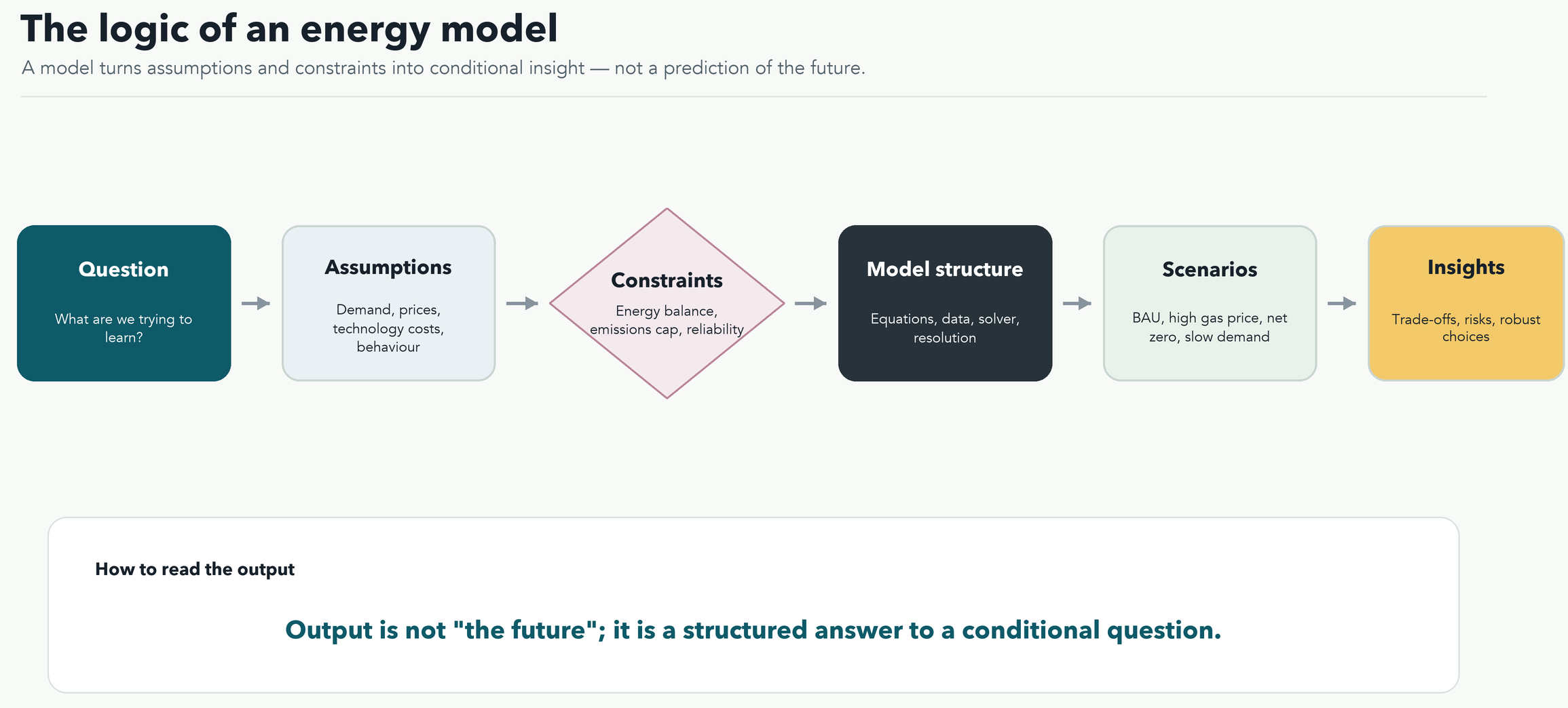
The best short description is: an energy model is a disciplined “what if?” machine. Not casual what-if thinking, where assumptions float around invisibly, but disciplined what-if thinking where the assumptions are written down, the flows have to balance, the constraints have to be respected, and the consequences can be compared.

But this is also why systems modelling matters. The energy transition is not a single-technology problem. It is a system transformation happening under planetary limits, social constraints, geo-political influence, uncertainty, and time pressure. Carbon, water, land, biodiversity, energy security, affordability, industrial competitiveness, poverty reduction, and intergenerational fairness can pull decisions in different directions. A system model gives analysts a sandbox for testing counterfactuals before choices are made in the real world: what if fuel prices rise, what if demand falls, what if storage becomes cheaper, what if carbon is capped, what if a technology arrives late, what if a transmission corridor is unavailable?

That sandbox is powerful because it can expose interactions that are hard to see from individual project analysis. A solar plant may look cheap by itself, but the system question asks what happens to grids, storage, dispatchable capacity, curtailment, demand flexibility, and market revenues when many solar plants are built. An electric vehicle may look like a transport technology, but at system level it is also a battery, a new electricity load, a demand-flexibility opportunity, a distribution-network challenge, and a policy problem.

Systems modelling is needed when the answer depends on how pieces interact.

Imagine the UK government asks:

If electricity demand rises, gas prices become volatile, carbon emissions must fall, and solar and batteries keep getting cheaper, what mix of generation, grids, storage, efficiency, and demand flexibility could meet demand at acceptable cost?

That question cannot be answered properly by opinion alone. It involves demand, capacity, hourly variation, geography, fuel prices, technology costs, emissions, reserve margins, infrastructure lead times, and policy constraints. A model does not remove judgement from the problem. It makes the judgement visible.

This is why many modelling lectures repeat a warning in different language: models are simplifications of reality, and their main value is insight. Energy planning is not about predicting the future. It is about evaluating possible futures in a transparent way.

Below I try to illustrate visually the logical steps of an energy model:

2. Define the energy system before defining the model

Before asking what an energy system model is, we need to ask what an energy system is.

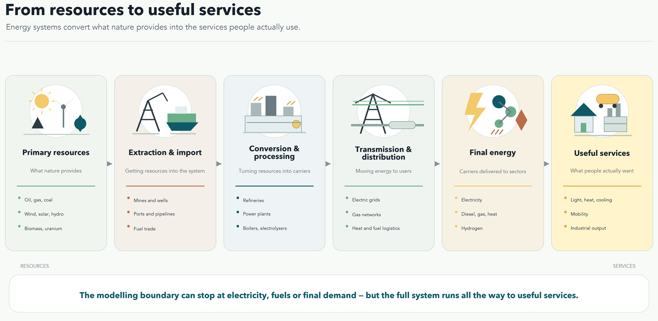
An energy system is the chain of resources, technologies, infrastructure, markets, and behaviours that converts what nature provides into what people want.

Nature provides coal, oil, gas, uranium, sunlight, wind, water flows, biomass, and geothermal heat. The energy sector extracts, imports, processes, converts, transports, stores, and distributes energy carriers. End-use technologies then convert those carriers into useful services.

The chain looks something like this:

Bad energy debates often start too late in the chain. They ask, “Should we build more solar or more gas?” before asking, “What services are we trying to provide, where, when, at what reliability, with what acceptable cost, and under what environmental constraint?”

The model boundary matters. A power-sector model might represent generation and electricity demand in detail but ignore industry, transport, buildings, land use, and macroeconomic feedback. A whole-system model might include all sectors but represent each with less engineering detail. An integrated assessment model might connect energy with land, emissions, climate, and the economy, but at a much higher level of abstraction.

There is no single correct boundary. There is only a boundary that is more or less fit for a question.

Example:

Suppose a household uses electricity for lighting, refrigeration, cooling, cooking, internet, and charging devices. If we model “electricity demand” as one block, we may miss the fact that some demand is flexible, some is seasonal, some is essential, some can be reduced by efficient appliances, some can move to another hour, and some is linked to weather. If the question is national annual fuel use, a simple electricity-demand block might be enough. If the question is grid stress during winter evenings, it is not.

3. Why energy systems need models?

Energy systems are hard to reason about because they combine five difficult properties.

First, they are physical. Electricity supply and demand must balance continuously. Fuels have energy contents. Conversion losses are real. A gas turbine cannot produce more than its capacity. A solar plant does not generate at night. A transmission line cannot carry infinite power.

Second, they are capital intensive. Power stations, refineries, pipelines, grids, storage facilities, buildings, industrial plants, and transport infrastructure require large upfront investment.

Third, they are long lived. A building, grid line, pipeline, refinery, or power plant can shape the system for decades. A decision made under today’s political and price conditions can still matter in 2050.

Fourth, they are socially embedded. A technically attractive system can fail if households reject it, investors avoid it, regulators block it, communities oppose it, or institutions cannot deliver it.

Fifth, they are uncertain. Future demand, fuel prices, technology costs, policy choices, climate impacts, social acceptance, geopolitical risks, and financing conditions are all uncertain.

This is why intuition alone fails. It may be obvious that a low-carbon energy system needs more renewables. It is not obvious how much grid reinforcement, storage, flexible demand, firm capacity, interconnection, hydrogen, district heat, industrial electrification, or energy efficiency is needed under a specific set of assumptions. It is not obvious whether a policy reduces emissions by shifting fuel use, lowering demand, changing investment, or merely moving emissions somewhere else.

Energy system models became important because they let analysts organise these interactions. They do not remove uncertainty, but they let us explore it. They do not replace politics, but they can clarify trade-offs.

Moreover, systems models let us study situations where real-world experimentation is impossible. They can be queried with counterfactual scenarios, sampled repeatedly for sensitivity to input data, or optimised for least cost, maximum resilience, or another objective. That is exactly the kind of tool needed when decision-makers face uncertain weather, uncertain policy, changing consumer preferences, volatile fuel prices, and infrastructure choices that last for decades.

Another reason models are needed is accountability. Without a model, a policy argument can hide its assumptions in prose: “renewables will be cheap”, “hydrogen will be available”, “demand will fall”, “gas will remain affordable”, “people will change behaviour”. A model forces these claims to become numbers, constraints, flows, costs, and scenarios. The model may still be wrong, but its wrongness becomes inspectable.

Finally, models are important because they influence investments and regulation.

Climate modelling makes this especially clear. The Coupled Model Intercomparison Project (CMIP), for example, coordinates common experiments across climate-modelling centres so that results can be compared and assessed; these projections are widely used in climate science and policy and underpin IPCC assessments.

Once CMIP model results enter assessments, regulation, finance, infrastructure planning, insurance, adaptation policy, and estimates of future climate damages to GDP, they become part of how governments and markets allocate real capital. Even critics of climate-scenario governance make the same deeper point: the choice of scenarios and modelling assumptions can influence research priorities, policy debates, regulation, and investment at enormous scale. This is why models are not just technical artefacts. When they inform decisions involving trillions of dollars, long-lived infrastructure, future economic damages, and public regulation, model design becomes a form of institutional power. Transparency, assumptions, validation, and scenario plausibility are therefore not academic housekeeping; they are central to responsible decision-making.

4. The energy trilemma and the modelling question

Modelling begins with a question, not software and you will never run out of questions!

Most energy-system questions sit somewhere inside the energy trilemma:

• Security: is supply reliable, sufficient, resilient, and geopolitically robust?

• Affordability: can households, firms, and governments pay for it?

• Environmental performance: does the system reduce greenhouse gases, local pollution, and other environmental harms?

These objectives are connected, but they are not identical. A system can be cheap and dirty. It can be clean and expensive. It can be secure but inefficient. It can be low cost in the model but politically impossible in practice. The modeller has to know which question is being asked.

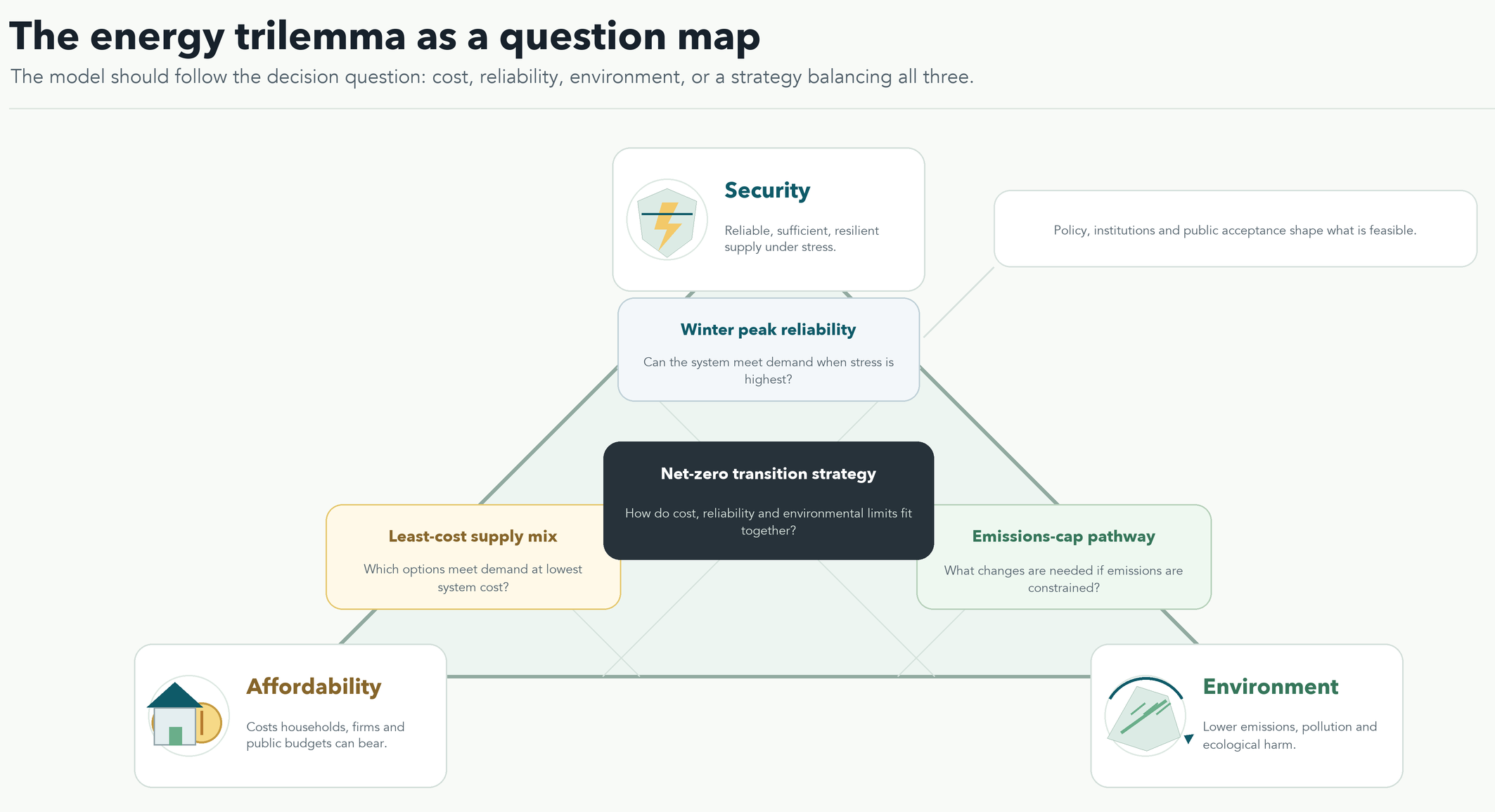
Consider three questions:

1. What is the least-cost electricity generation mix?

2. What system can meet winter peak demand reliably?

3. What policy package is politically and institutionally feasible?

These are not the same modelling problem. The first might be answered with a long-term capacity expansion model. The second may need detailed temporal resolution and reliability constraints. The third may require political economy, stakeholder engagement, behavioural assumptions, and institutional realism.

Example: Three valid questions, three different models

For decarbonising heat:

• An engineering model may ask which heat technologies can technically satisfy heat demand.

• An economic model may ask how prices, subsidies, or fuel taxes influence adoption.

• A behavioural model may ask whether households accept disruption, upfront costs, and perceived risk.

All three are useful. None is complete alone.

5. The main families of energy models

Once the system and question are clear, we can talk about model families.

At the highest level, energy models are often described as top-down, bottom-up, or hybrid.

Top-down models start from the economy. They represent broad sectors and macroeconomic relationships, often using input-output structures, econometrics, or general equilibrium methods. They are useful for questions about GDP, prices, income, competitiveness, sectoral feedback, and economy-wide policy effects. Their weakness is that they often represent energy technologies in less physical detail.

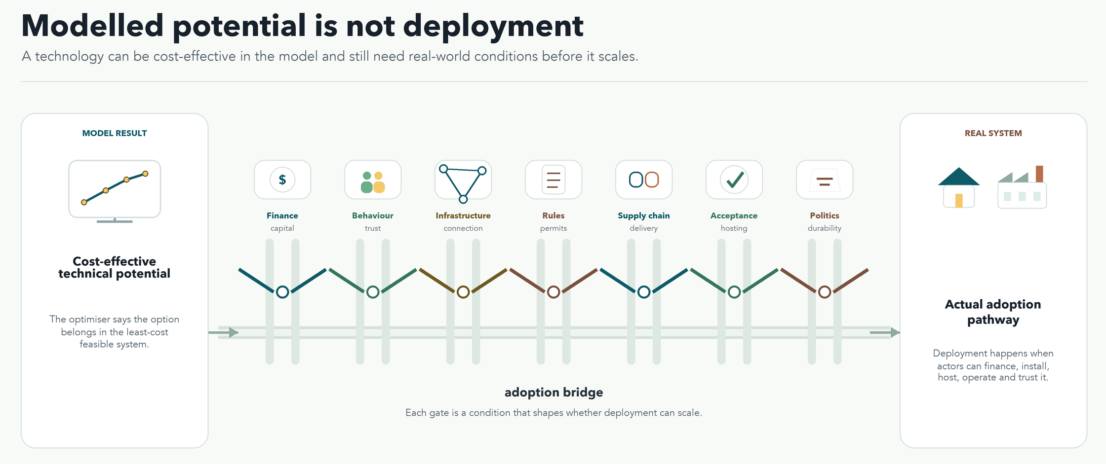
Bottom-up models start from technologies and energy flows. They represent power plants, vehicles, boilers, industrial processes, fuels, conversion efficiencies, costs, emissions, and resource potentials. They are useful for studying technology choices, infrastructure pathways, emissions reduction, and system costs. Their weakness is that they can be too optimistic if they assume technologies are adopted whenever they are cost-effective, ignoring behavioural and institutional barriers.

Hybrid models try to link the two: technological detail from bottom-up models with wider economic feedback from top-down approaches. The ambition is attractive. The implementation is difficult.

Models can also be grouped by method:

• Accounting models describe energy balances and emissions under user-defined assumptions.

• Simulation models reproduce system behaviour under decision rules.

• Optimisation models select decisions that maximise or minimise an objective under constraints.

• Equilibrium models solve for a state where interacting agents or markets balance supply and demand.

• Dispatch models focus on short-term operation.

• Capacity-expansion or investment models focus on long-term build-out.

• Integrated assessment models (IAMs) link energy, economy, land, emissions, and climate outcomes.

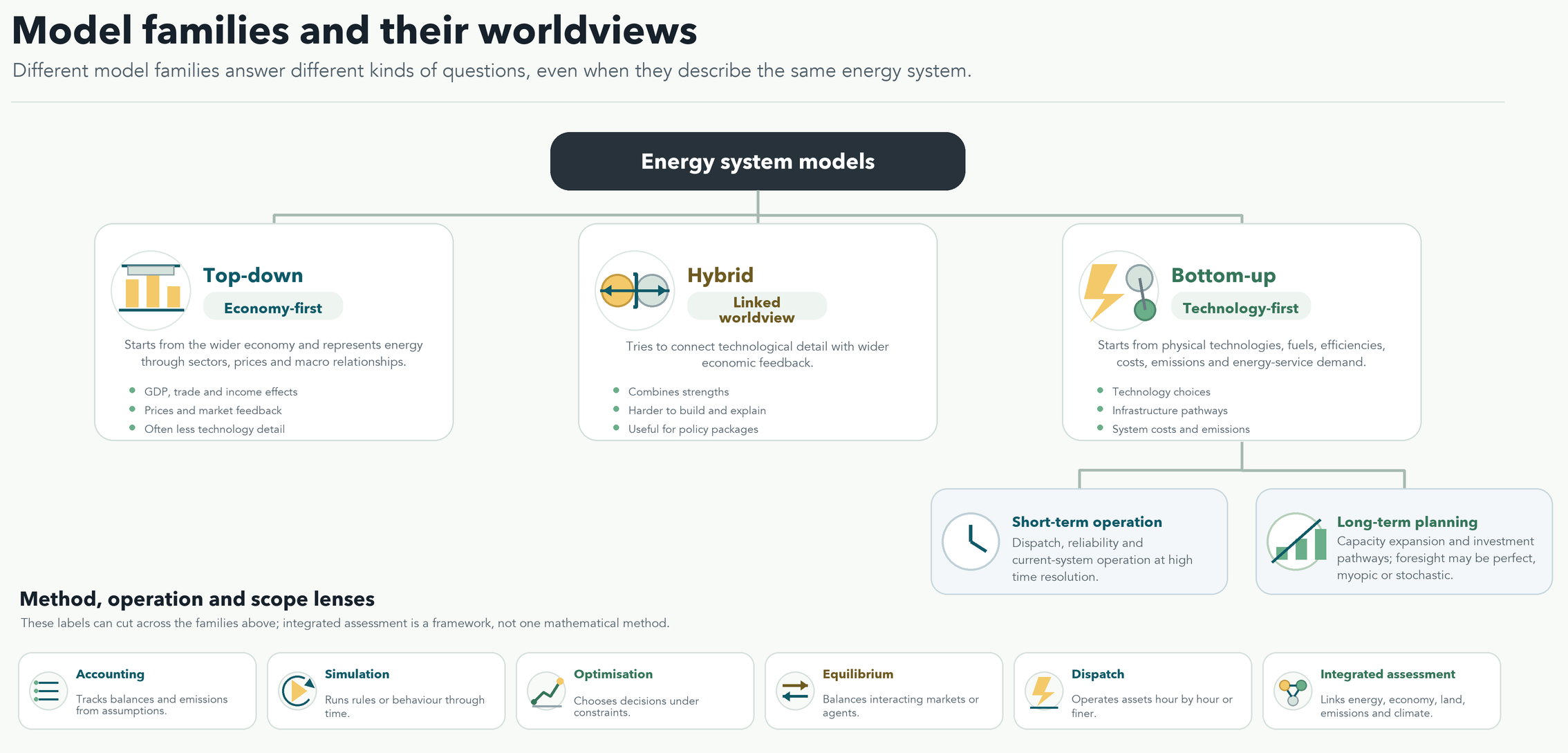
When a bottom-up optimiser says a technology is chosen, it usually means the technology helps satisfy the objective and constraints. When an equilibrium model gives a price, it reflects a representation of market balance. When an accounting model shows an emissions pathway, it may be applying externally chosen activity and technology assumptions. When an IAM shows a 1.5C pathway, it is linking energy and land transformations to climate outcomes under a wider scenario structure.

There is a second layer to model families that is just as important: model design. This is especially visible in bottom-up and many hybrid models. A model can be bottom-up and still be very different depending on whether it covers one sector or all sectors, one country node or many connected regions, annual periods or hourly operation, simulation or optimisation, linear or nonlinear equations, perfect foresight or myopic decision-making.

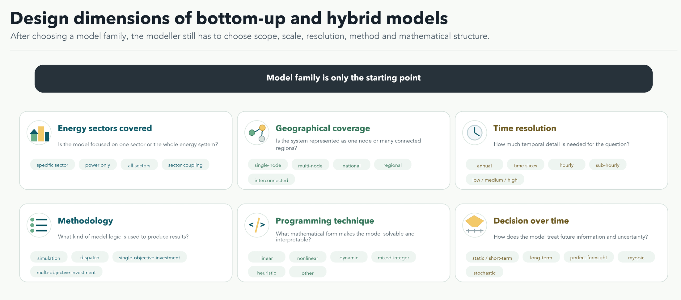
These specifications decide what the model can see. A single-node model may be useful for national planning but weak for transmission bottlenecks. An annual model may be useful for long-term investment but weak for solar, wind, storage and peak demand. A perfect-foresight model may identify a clean long-term pathway but may overstate how much decision-makers know today. A mixed-integer formulation may represent yes/no decisions more realistically but may be harder to solve at large scale.

There is also a historical story here. Energy system modelling did not appear because academics wanted complicated diagrams. It grew out of practical crises and planning needs.

The early 1970s oil shocks pushed governments and research institutions to think systematically about fuel allocation, energy security, and uncertain futures. Reference Energy System ideas were developed at Brookhaven National Laboratory, and linear programming approaches helped represent energy flows and technology choices.

During the 1980s, models such as EFOM, MARKAL, MAED, and later TIMES helped formalise energy demand, supply, and power-sector planning.

In the 1990s, market-oriented and equilibrium models such as PRIMES and NEMS expanded the modelling landscape. Later, rising concerns about climate change, energy security, prices, and global demand pushed models toward wider sector coverage, long-term decarbonisation pathways, open-source tools, and fit-for-purpose design.

Example: The same policy seen by different model families

A carbon price can appear very differently across models:

• In a bottom-up optimisation model, it changes relative technology costs and may shift investment.

• In a top-down model, it can affect prices, income, output, trade, and sectoral structure.

• In a hybrid model, it may shift both technology deployment and macroeconomic outcomes.

• In an IAM, it may be part of a pathway linking emissions to temperature outcomes.

6. Energy balance and flows

Before there is optimisation, there is accounting or baselining.

Energy models must represent physical flows. Resources enter the system. Conversion technologies transform them. Losses occur. Energy carriers move through networks. Final energy reaches sectors. Useful services are produced.

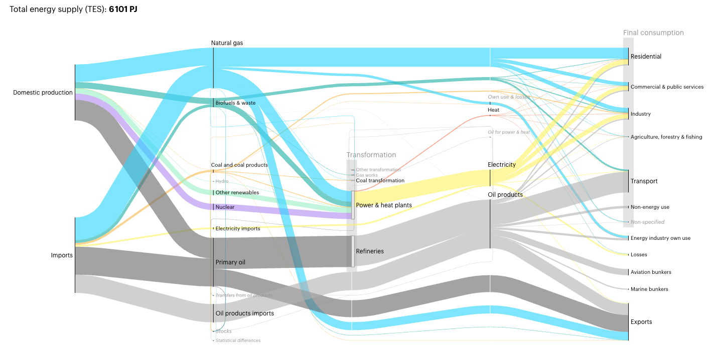
This physical skeleton is often represented through an energy balance or a reference energy system. A Sankey diagram usually visualises the size of flows, making it easier to see where energy comes from, where it goes, and where it is lost.

Energy systems obey physical constraints. The first law of thermodynamics is not a policy preference. Energy is converted, not created from nothing. A power plant converts fuel into electricity and losses.

Modelling begins by respecting this skeleton.

Example: Oil, gas, electricity, and useful services

Oil may be refined into petrol, diesel, kerosene, or fuel oil. Gas may go to power generation, industry, heating, or feedstock. Electricity may serve buildings, industry, transport, and communications. Some energy is lost in conversion and networks. Some is transformed into useful work, heat, cooling, or light. A Sankey diagram lets the reader see this in one image.

For reference, this is the UK’s system balance in 2023 which can be used as the baseline for system modelling (source IEA, interactively here).

7. The mathematical core

Now we can open the mathematical box, which is the heart of energy system modelling.

A model usually contains:

• Variables: things the model can choose or calculate.

• Parameters: input assumptions given to the model.

• Constraints: rules that must be satisfied.

• An objective function: something to minimise or maximise (for optimisation models)

In many bottom-up energy-system optimisation models, the objective is to minimise total discounted system cost while meeting energy-service demand and respecting constraints.

The cost might include capital investment, fixed and variable operation and maintenance, fuel purchases, imports, taxes, subsidies, carbon prices, emission penalties, and other system costs. The constraints might include demand satisfaction, capacity limits, resource potentials, capacity factors, reserve margins, emissions caps, build-rate limits, technology lifetimes, storage balance, and policy targets.

That sounds abstract, so let us start with a carpenter.

Example 1: The carpenter problem

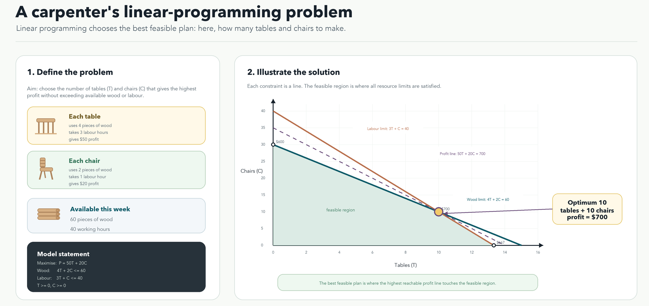
A carpenter can make chairs and tables. A table uses 4 pieces of wood, takes 3 hours to make, and gives $50 profit. A chair uses 2 pieces of wood, takes 1 hour to make, and gives $20 profit. This week, the workshop has 60 pieces of wood and 40 working hours.

The question is simple: how many tables and chairs should the carpenter make so that wood and labour are not exceeded, while total profit is as high as possible?

This is a linear programming problem. The decision variables are the number of chairs and tables. The constraints are wood and labour. The objective is profit. The feasible region is the set of production combinations that do not exceed the available resources. The optimum is the best point inside that feasible region.

Let:

T = number of tables
C = number of chairs

The model is:

Maximise profit: P = 50T + 20C

Subject to:
Wood: 4T + 2C <= 60
Labour: 3T + C <= 40
T >= 0, C >= 0

Graphically, each constraint becomes a line. The area that satisfies both constraints is the feasible region. The best answer is the feasible point reached by the highest profit line. In this example, the optimum is 10 tables and 10 chairs, giving:

Profit = 50(10) + 20(10) = $700

Example 2: The energy-system equivalent

A national electricity system can build solar, wind, gas, batteries, grid reinforcement, and efficiency. Solar and wind have variable output. Gas has fuel cost and emissions. Batteries shift electricity but do not create it. Grid reinforcement allows remote generation to reach demand. Efficiency reduces useful energy requirements. The system must meet demand, respect emissions limits, satisfy reliability requirements, and stay within technology/resource limits.

Now the variables are capacity, generation, storage charge/discharge, fuel use, imports, and perhaps demand reduction. The constraints are energy balance, capacity availability, emissions, reserves, resource limits, and policy rules. The objective might be least total discounted cost.

This is why “the model chose solar” is shorthand. More precisely, the solution found that, under the assumed costs, resources, demand, policy constraints, and mathematical structure, solar capacity was part of the least-cost feasible system.

Tiny illustrative code snippet

This is not the article’s main teaching device, but a small code box can help readers see that optimisation is not magic:

# Toy resource-allocation problem

# Maximise profit from chairs and tables subject to wood and labour.

import pulp as pl

model = pl.LpProblem("carpenter", pl.LpMaximize)

tables = pl.LpVariable("tables", lowBound=0)

chairs = pl.LpVariable("chairs", lowBound=0)

# Profit per unit

model += 50 * tables + 20 * chairs

# Resource constraints

model += 4 * tables + 2 * chairs <= 60 # wood

model += 3 * tables + chairs <= 40 # labour

model.solve()

print(tables.value(), chairs.value(), pl.value(model.objective))

Then translate the same logic:

chairs/tables -> solar/wind/gas/storage/efficiency
wood/labour -> land/resource/capital/grid/fuel limits
profit -> cost, emissions, or welfare objective
production mix -> energy-system pathway

Why linearity matters?

Many energy-system models are formulated as linear or mixed-integer linear programmes. That is not only a mathematical preference. It is a practical compromise.

Linear models are attractive because they can be solved efficiently and, in many cases, exactly. The solver can prove that it has found the best solution according to the objective and constraints. Linear models are also memory-efficient enough to represent large systems with many technologies, regions, time periods, commodities, and constraints. That is one reason they became so important in energy planning.

But linearity has consequences.

In a linear model, marginal costs are usually constant unless the modeller adds piecewise segments. Economies of scale, learning, congestion, market power, profitability, price formation, and strategic behaviour are not automatically represented. If cost is linear, doubling output doubles variable cost. If a technology has a nonlinear cost curve, the modeller has to approximate it. If price depends on quantity, and revenue is price multiplied by quantity, that multiplication is nonlinear and cannot simply be dropped into a linear model without reformulation.

This matters for interpretation. A least-cost investment model may build a large amount of zero-marginal-cost renewable capacity because it reduces system cost. But in an actual market, that same build-out can reduce wholesale prices during sunny or windy hours and erode the revenues of the very assets the model builds. The system-cost optimum and the private-investor business case are not always the same object.

So linearity is a bargain: it gives tractability, scale, and clear optimisation, but it asks the modeller to be honest about what economic and physical behaviour has been simplified. A linear model is not weak because it is linear. It becomes weak when readers forget what linearity excludes.

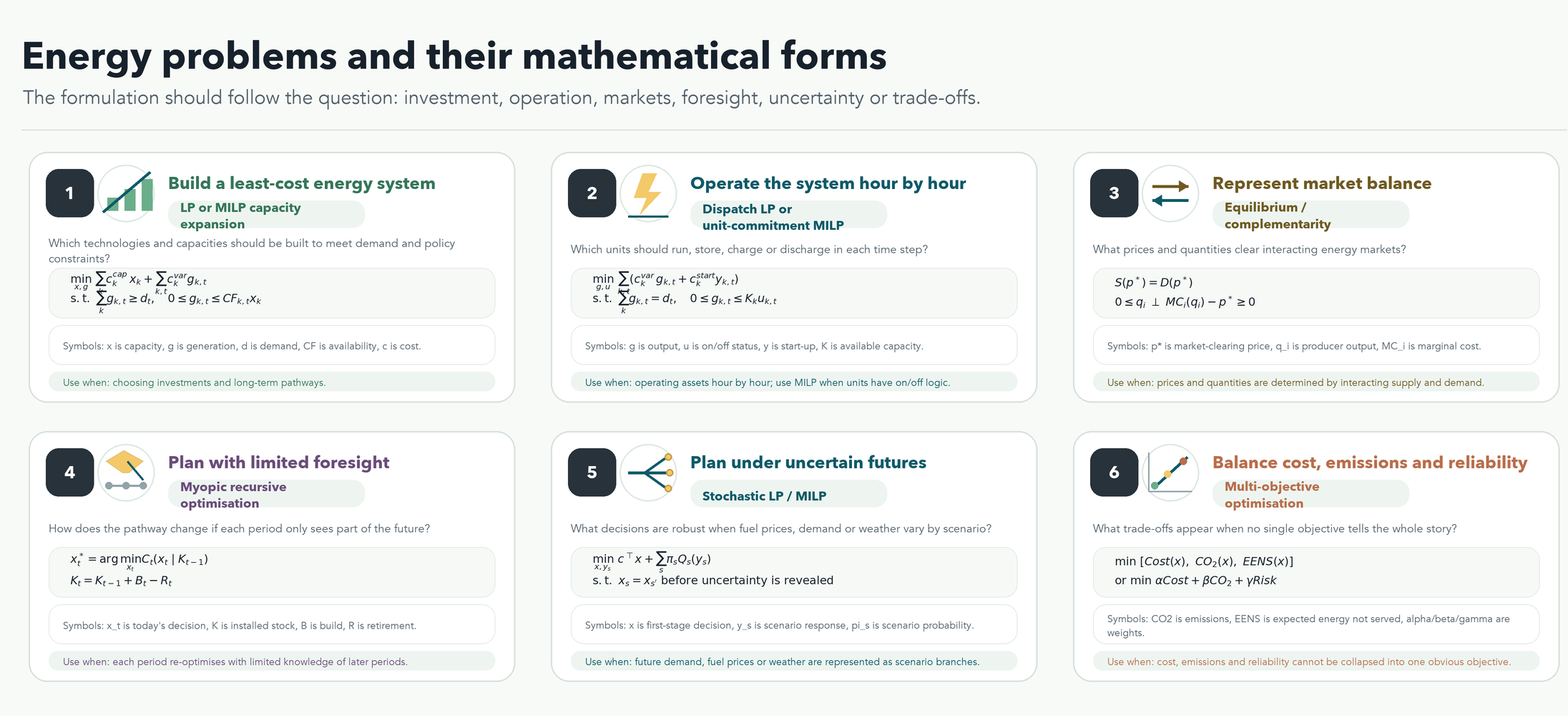
The carpenter example shows the basic optimisation logic. Real energy-system questions then branch into several mathematical forms (see below). The formulation follows the question:

• If the question is “what should we build?”, the formulation is often capacity-expansion optimisation.

• If the question is “what should run this hour?”, it is often dispatch or unit commitment.

• If the question is “what price clears the market?”, equilibrium or complementarity methods may be appropriate.

• If the question is “what would decision-makers do with limited foresight?”, a myopic recursive formulation may be used.

• If the question is “what if the future branches?”, stochastic optimisation may be used.

• If the question has competing objectives, multi-objective methods or Pareto analysis may be needed.

8. The resolution problem

The most detailed model is not automatically the best model.

Every model has a resolution. It can be high or low in time, space, technology detail, sector coupling, and behaviour. A modeller cannot represent everything at maximum detail without paying a price in data, computation, validation, and communication. The skill is deciding where fidelity matters for the question.

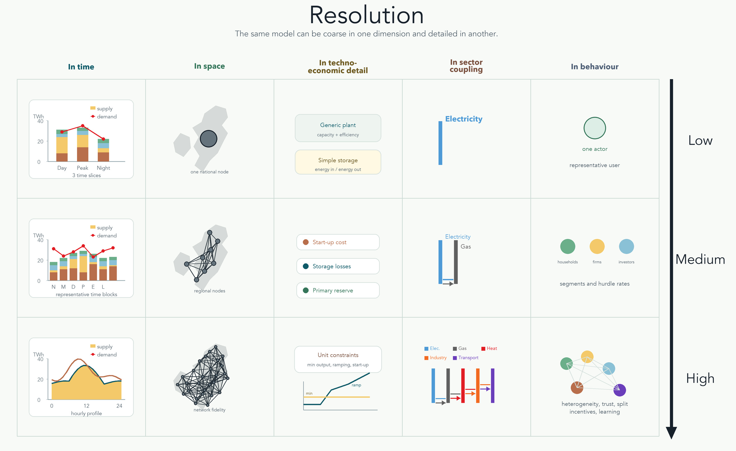
Temporal resolution asks: does the model see annual totals, seasons, representative days, hours, or sub-hourly operation?

Spatial resolution asks: does the model treat the world as one region, a country as one node, a country as several zones, or a grid as many connected buses? Many system models are built as networks of nodes. A node might represent a real geography, such as a country, province, grid zone, industrial cluster, port, or demand centre. It can also represent a figurative market node, such as an import/export market.

Technology resolution asks: does the model have one generic “gas plant” or distinguish open-cycle turbines, combined-cycle plants, CHP, hydrogen-ready turbines, plant vintages, efficiencies, ramping limits, and emissions rates?

Sectoral resolution asks: does the model cover only electricity, or electricity plus heat, transport, buildings, industry, hydrogen, land, and fuels?

Behavioural resolution asks: does demand respond mechanically to prices, or are households, firms, and institutions represented with heterogeneity and non-cost barriers?

Higher resolution can reveal things that lower resolution hides. Hourly modelling can show the value of storage, flexibility, and firm capacity in a renewable-heavy power system. Spatial modelling can show grid bottlenecks. Sector coupling can show the interaction between electric vehicles, heat pumps, hydrogen, and power demand. High technical detail can distinguish a flexible gas turbine from an inflexible coal plant, or a generic steel plant from a specific route such as blast furnace/basic oxygen furnace versus direct reduced iron/electric arc furnace.

But detail has costs. It requires data, computation, interpretation, and discipline. More detail can make a model harder to validate, harder to explain, and easier to mistake for reality. Sometimes a simpler model is more useful because it answers the question cleanly.

The right question is not “how detailed can we make it?” The right question is “what level of detail is necessary for this decision?” For a model of annual industrial transition, five-year time steps may be reasonable. For power-system operations with variable renewables, hourly or sub-hourly time may be essential. For a national strategy, one node may be enough for a first pass. For transmission planning, one node is almost certainly misleading.

9. The economics

Most energy models we use today are often described as “least-cost” models. But this is only the doorway into the economics. Under the surface, models are dealing with a deeper question:

How should scarce resources be allocated to produce energy services?

That question is economic before it is mathematical. There is demand: people, firms and institutions want heat, cooling, mobility, light, industrial output and digital services. There is supply: technologies, fuels, networks, storage, labour, capital, land, water and materials. There are constraints: physics, capacity, emissions, reliability, build rates, geography, policy and money.

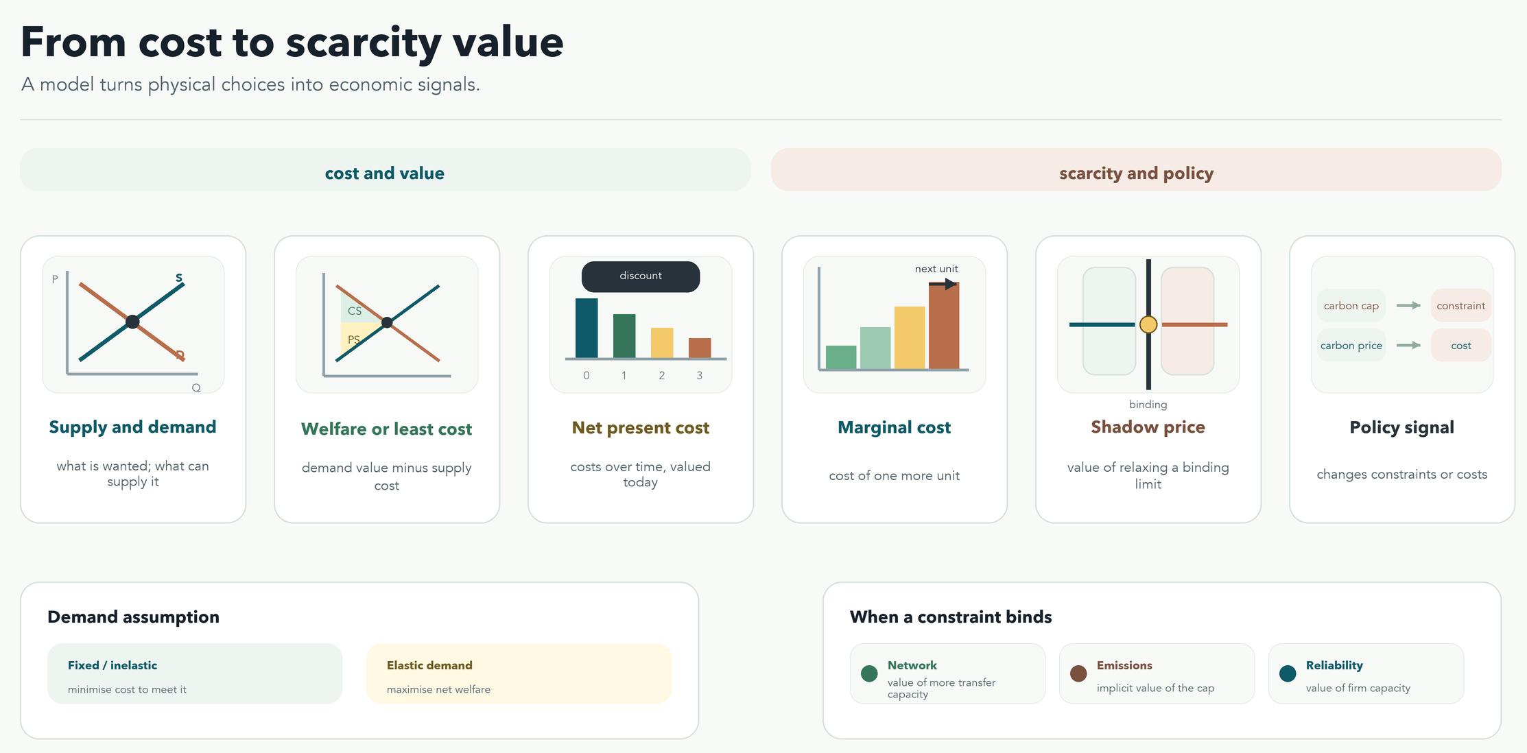
A simple supply-and-demand diagram is therefore not a distraction from energy-system modelling. It is one of its foundations. A supply curve says what it costs to provide more of something. A demand curve says what consumers are willing to pay, or how much they value another unit. Where supply and demand meet, a market-clearing quantity and price can emerge. In a real energy system, this happens across many fuels, sectors, locations and time periods at once.

This is why energy models can look like engineering tools but still behave like economic machines.

Least cost is a special case

In economics, demand can be elastic or inelastic. Elastic demand changes noticeably when price changes. Inelastic demand changes little, at least in the short run. Electricity demand, for example, is often relatively inelastic over short periods because households and firms still need heat, cooling, light, refrigeration and production. Many least-cost energy models go one step further: they treat demand as fixed or exogenous. The model must meet it, whatever the implied cost. Other models allow demand to respond through efficiency, demand response, fuel switching or reduced service demand.

Many bottom-up energy models take energy-service demand as fixed. In that case, the model does not ask whether society wants more or less of the service. It accepts the demand as an input and asks:

What is the lowest-cost way to meet this demand while respecting all constraints?

In plain terms:

Minimise total system cost
subject to demand being met,
technologies operating within limits,
emissions staying within limits,
and all other constraints being respected.

That is powerful, but it is not the whole economic story. If demand is allowed to respond to price, then the model can ask a wider welfare question:

Maximise net social welfare
= value of energy services to consumers
- cost of supplying those services
- external costs not already priced

In this language, welfare means net economic value. Consumer surplus is the value consumers receive above what they pay. Producer surplus is the value producers receive above their cost. Some equilibrium models, including TIMES-style formulations, can be interpreted through this total-surplus logic. When demand is fixed, welfare maximisation often collapses into a cost-minimisation problem because the value of demand is no longer changing inside the model.

This distinction matters. A model with fixed demand may conclude that a very expensive system is required to meet a given level of service. A model with elastic demand may instead show that some demand reduction, efficiency, demand response or behavioural change is economically valuable. The difference is not a modelling trick. It is a different representation of the demand side.

Net present cost

Energy investments happen over time. A gas plant, wind farm, transmission line, refinery, building retrofit or heat network may create costs and benefits for decades. The model therefore needs a way to compare money spent today with money spent or saved in the future.

That is where discounting enters.

The discount factor for year y is:

discount factor = 1 / (1 + r)^y

where r is the discount rate. A higher discount rate gives less weight to future fuel savings, future emissions reductions and future operating-cost benefits. A lower discount rate gives the future more weight.

For a system model, the net present cost can be written in plain language as:

Net present system cost =
discounted capital cost
+ discounted fixed O&M
+ discounted variable O&M
+ discounted fuel cost
+ discounted emissions cost
+ discounted policy or penalty costs
- discounted salvage value

This is why financing assumptions can change model results. A technology with high upfront cost and low operating cost, such as wind, solar, nuclear, grids or efficiency, is sensitive to the cost of capital. A technology with lower upfront cost but ongoing fuel exposure is sensitive to fuel price, carbon price and utilisation. “Cheapest” is not a property sitting inside the technology. It is a result of time, finance, fuel, utilisation, policy and system context.

Levelised cost is one useful shortcut, but it is an average-cost metric, not a full model of system value:

Levelised production cost =
discounted lifetime cost / discounted lifetime useful output

This can help compare similar technologies, but it can mislead when technologies provide different services. One MWh at midday is not always worth the same as one MWh on a cold, dark, windless evening. A cheap generator in a constrained location may be less valuable than a more expensive resource near demand. A plant with a higher average cost may still be valuable if it provides firm capacity, flexibility, inertia, heat, hydrogen, reserves or security of supply.

The model’s job is to place cost inside the system, not treat it as an isolated number.

Marginal cost: the cost of one more unit

Average cost asks: what does this technology cost per unit over its lifetime?

Marginal cost asks: what is the cost of one more unit now?

That difference is central to energy modelling. In electricity dispatch, the marginal generator is the next plant needed to meet demand. If wind and solar are available, their short-run marginal cost may be close to zero. If the system then needs a gas turbine, the marginal cost includes fuel and variable operating cost. If the system is short of capacity, the marginal value of demand response, storage, imports or firm generation can rise sharply.

For a simple dispatch model, the economic logic is:

Use the lowest marginal-cost resources first,
then use more expensive resources as demand rises,
until demand is met.

This is the merit-order idea. But modern systems complicate it. The marginal unit may depend on network congestion, ramping limits, storage state of charge, weather, reserve requirements, emissions constraints and unit-commitment decisions. The marginal cost in one location and hour may differ from another location and hour.

This is where modelling starts to reveal scarcity.

Shadow prices: the value of relaxing a constraint

One of the most useful outputs of an optimisation model is not only what it builds or dispatches. It is what the constraints are worth.

In a linear optimisation model, each constraint has an associated dual value, often called a shadow price. In practical language:

Shadow price =
how much the objective would improve
if a binding constraint were relaxed by one unit.

If a constraint is not binding, its shadow price is usually zero. The system has room. Relaxing the constraint does not help. If a constraint is binding, the shadow price tells you that the system is being held back by that limit.

The shadow price of an electricity balance constraint can be interpreted as the marginal cost of serving one more unit of demand at a specific node and time. In market language, this is closely related to a locational marginal price.

The shadow price of an emissions cap can be interpreted as the implicit value of one more tonne of allowed emissions. If the cap is tight, relaxing it may reduce system cost. That shadow price is not automatically a politically chosen carbon price, but it tells you what carbon constraint the model is feeling.

This is why shadow prices are so useful for policy and planning. They tell the analyst where scarcity is actually appearing in the model. The bottleneck may not be the technology everyone is arguing about. It may be the grid, winter peak, industrial heat, build rate, flexibility, finance, land, emissions or institutional constraint.

There is one important caution. Shadow prices are cleanest in linear programming. In mixed-integer models, where decisions such as unit commitment or lumpy investment are represented with integer variables, dual values need more care. The broad interpretation still matters, but the modeller must not report shadow prices mechanically without understanding the formulation.

Example: A winter evening

Imagine a winter evening in 2035. Demand is high. Solar output is gone. Wind output is low. Gas prices are high. A transmission line into the demand centre is congested. The emissions cap is nearly binding. Batteries are partly discharged.

A model result might say: build more storage, keep some firm capacity, reinforce the grid, and reduce peak demand through flexibility.

The cost table alone will not explain why. The economics inside the model will.

The marginal cost of serving one more MWh is high because the next available resources are expensive. The transmission shadow price is high because congestion is preventing cheaper supply from reaching demand. The emissions shadow price is high because fossil backup is constrained. The reserve constraint may show a high value for firm capacity. The model is not simply saying “storage is cheap” or “gas is expensive”. It is revealing a pattern of scarcity across time, space, emissions and reliability.

10. Markets, policy, and model closure

Energy systems are shaped by policy and markets. Models have to represent that somehow.

A policy can enter a model as a target, a constraint, a price, a subsidy, a standard, or a behavioural assumption.

An emissions cap can force total emissions below a limit. A carbon tax can increase the cost of emissions-intensive fuels and technologies. A renewable target can require a minimum share or quantity of renewable generation. A subsidy can reduce the apparent cost of a technology. Efficiency standards can reduce demand or change technology availability. A price cap can affect revenues, investment, and market behaviour if the model represents them.

The same physical system can produce different results under different policy representations.

Markets are one way an energy system decides who builds, who operates, who pays, and who receives revenue. A model may represent the system as if a single planner minimises total cost, or it may represent decentralised decisions through prices, market clearing, tariffs, subsidies, contracts and regulations. These are not equivalent assumptions. A least-cost pathway may show what would be efficient for the system as a whole, but a real market asks whether investors can recover costs, whether consumers face the right prices, whether network charges are designed well, and whether policy rules make the modelled pathway financeable.

Model closure is the set of assumptions that makes the model solvable. What is exogenous? What is endogenous? Is demand fixed or price-responsive? Are fuel prices given externally or produced by a market module? Can the country import unlimited fuel at a fixed price, or is trade constrained? Are investors assumed to minimise social system cost, private cost, or something else? Are technologies available instantly, or limited by build rates and supply chains?

These choices are not technical footnotes. They shape the answer.

Example: Four policy levers, four model effects

• Carbon cap: emissions cannot exceed a limit.

• Carbon tax: emitting technologies become more expensive.

• Renewable target: renewable deployment must reach a required level.

• Capital subsidy: selected technologies become cheaper to build.

Each can reduce emissions, but each works through a different model mechanism.

11. Behaviour, barriers, and the real world outside the equation

If energy system modelling stops at techno-economic optimisation, it misses much of the real world.

Energy transitions are not implemented by a single benevolent planner with perfect information and infinite political authority. They are implemented through households, firms, investors, regulators, ministries, grid companies, local communities, supply chains, banks, and politicians. These actors have different incentives, risk perceptions, time horizons, capabilities, and constraints.

A least-cost model may assume a technology is adopted because it is cost-effective. Real households may not adopt it because the upfront cost is high, the payback is uncertain, the installation is disruptive, the landlord pays while the tenant benefits, information is poor, trust is low, or the technology is unfamiliar. Real investors may avoid a technology because of policy risk, currency risk, offtake risk, fuel risk, or uncertainty over future market rules.

Behavioural modelling tries to represent some of this. It may use hurdle rates, market heterogeneity, replacement rates, demand elasticities, intangible costs, or segmented actors. These are imperfect, but they are attempts to avoid pretending that every actor behaves like the optimiser.

Social barriers also matter. Public acceptance, planning permission, land use, visual impacts, local disruption, and trust can shape technology deployment. Infrastructure lock-in matters too. An existing grid may have been built around centralised power stations, not distributed renewable generation. A city may have been built around private cars, not public transport or walkability.

Example 1: The EV charging loop

Few people buy electric vehicles if charging infrastructure is weak. But firms may not build charging infrastructure if few people have electric vehicles. The system can get stuck. Policy can break the loop by supporting early infrastructure, reducing risk, or coordinating investment.

Example 2: Wind variability as a multi-dimensional barrier

Variable wind output is a technical issue because supply changes with weather. It is an economic issue because backup, storage, grids, and flexibility cost money. It is a social issue because people value reliability and may resist infrastructure. It is a political issue because asking people to use electricity only when the wind blows is usually unacceptable. One barrier can sit across technical, economic, social, and political categories at once.

12. Scenarios and Uncertainty

A scenario is an internally consistent story translated into assumptions. It may describe high demand growth, rapid technology learning, strong climate policy, weak policy, high fuel prices, low fuel prices, fast electrification, slow behavioural change, or different socio-economic futures.

Sensitivity analysis is different. It changes one or a small number of inputs to see how results respond. What happens if gas prices are 30 percent higher? What happens if battery costs fall faster? What happens if demand is lower? Sensitivity analysis is useful because it shows which assumptions matter.

Scenario analysis changes a coherent package of assumptions. For example, a “strong climate policy” scenario might combine an emissions cap, high carbon price, faster electrification, renewable support, and efficiency measures. A “high fossil fuel price” scenario might affect dispatch, investment, imports, and end-use technology choices. A “slow demand growth” scenario might reduce capacity needs and investment pressure.

Stochastic modelling goes further by representing uncertain future branches with probabilities. Myopic modelling represents decisions made without full knowledge of future assumptions. Perfect-foresight modelling assumes future conditions are known across the model horizon( i.e, the model knows what to choose in advance) . Each approach represents a different view of decision-making under uncertainty.

The critical habit is to read results with the assumptions attached. A model result without its scenario assumptions is like a map without a scale.

Example: Four futures, four pathways

Compare four scenarios:

• High fossil fuel prices.

• Low renewable and storage costs.

• Slow demand growth.

• Strong climate policy.

Each can produce a different pathway. High fuel prices may favour efficiency and renewables. Low renewable costs may accelerate electrification. Slow demand growth may reduce new-build requirements. Strong climate policy may force early retirement or reduced operation of high-emission assets.

13. Integrated assessment models

IAMs place energy-system change inside a wider climate-policy framework.

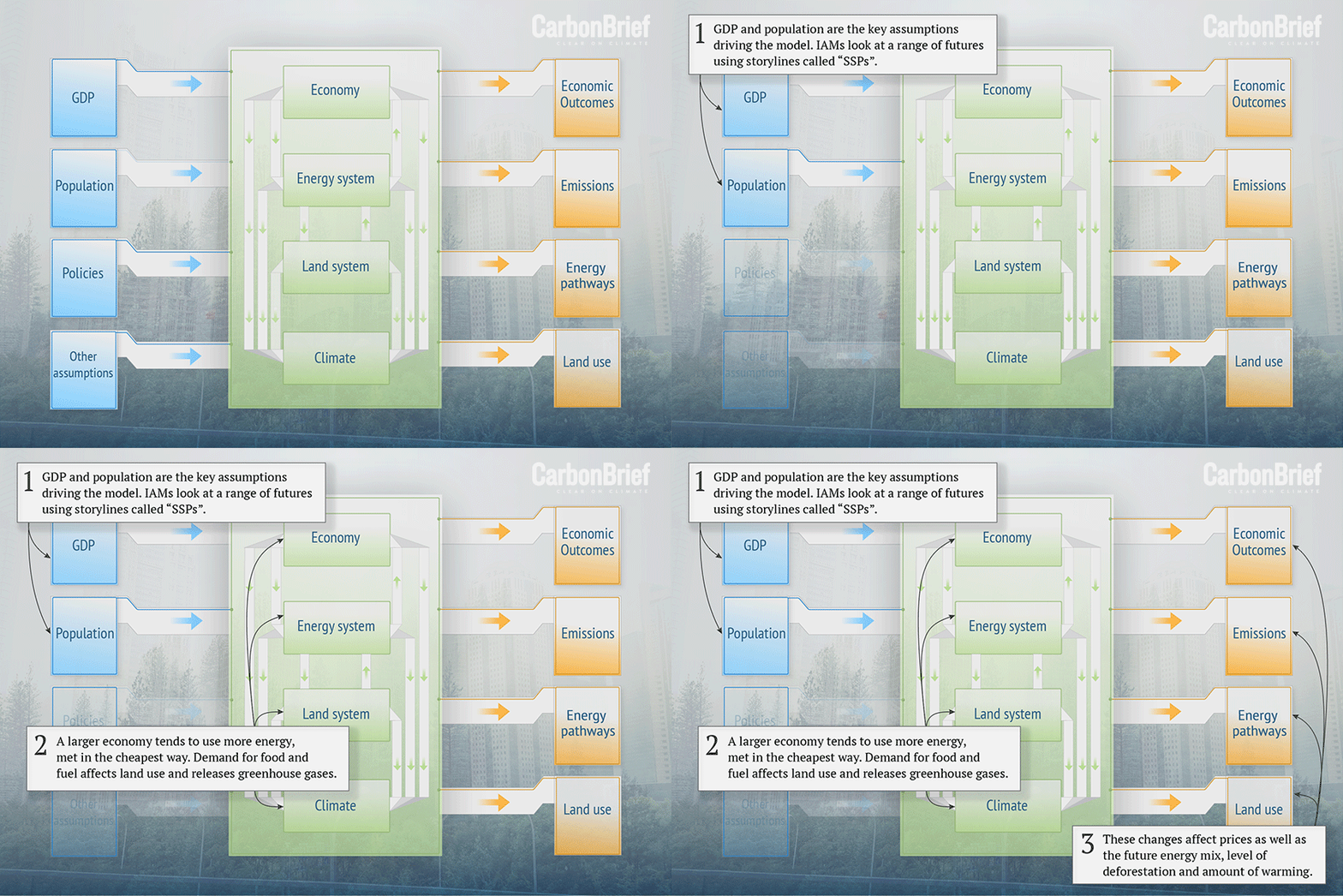
They are “integrated” because they link multiple systems: energy, economy, land use, emissions, and the climate. They are used to study questions such as how the world might limit warming to 1.5C or 2C, how emissions pathways differ under policy assumptions, and what combinations of energy transformation, land-use change, negative emissions, and demand change could be consistent with climate goals.

IAMs matter because many global climate pathways including IPCC ones, including those assessed in climate-policy debates, come from them. They allow researchers to connect human development, energy use, land systems, emissions, and temperature outcomes in one framework.

But IAMs are not magic. They are simplified representations of very complex systems. They may represent some technologies, behaviours, or political constraints imperfectly. They may rely on assumptions about future demand, technology learning, carbon dioxide removal, land availability, bioenergy, electrification, and policy coordination. Different IAMs can agree on broad directions while disagreeing on details.

This does not make IAMs useless. It means they must be read as structured scenario tools, not as destiny. Their value is in clarifying what kinds of transformations are implied by climate goals and where assumptions matter most.

Example: A 1.5C pathway

A pathway compatible with 1.5C may involve rapid emissions reductions, electrification, energy efficiency, renewable deployment, changes in land use, reduced fossil fuel use, and some level of carbon dioxide removal.

If a pathway relies heavily on negative emissions later, the reader should ask: how much, from which technologies, with what land and energy requirements, and what happens if deployment is slower?

This interactive figure from CarbonBries explains how IAMs work for one scenario (source)

14. How models are built in practice

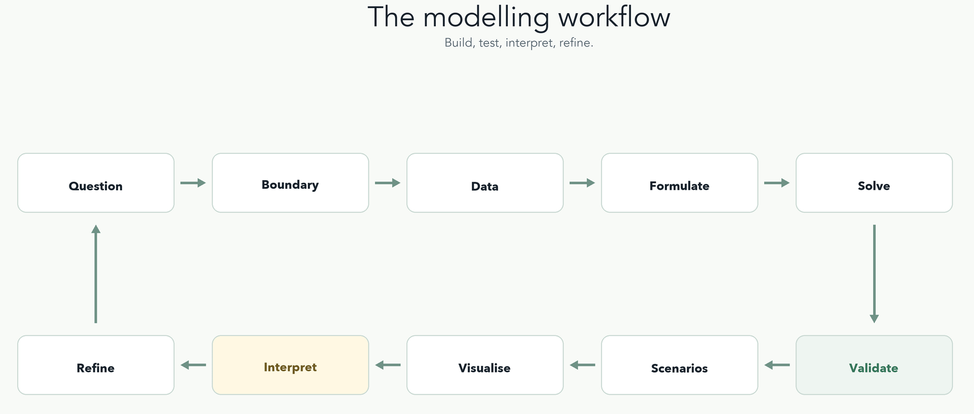
The modelling workflow is less glamorous than the final charts suggest.

It usually looks like this:

1. Define the question.

2. Define the system boundary.

3. Decide the model type and level of detail.

4. Gather raw data.

5. Process data into consistent formats.

6. Build the reference system or base-year balance.

7. Formulate equations, variables, constraints, and objective.

8. Implement the model in software.

9. Solve the base case.

10. Test and validate behaviour.

11. Build policy or uncertainty scenarios.

12. Post-process results.

13. Interpret results for the decision.

14. Revise assumptions and repeat.

The iteration is important. A model is rarely built perfectly from the start. A good modeller starts simple, checks whether the model behaves sensibly, then adds complexity only when it is needed.

This is also where transparency matters. The model should document data sources, assumptions, equations, scenario definitions, and limitations. If other people need to use or trust the model, the workflow cannot live only in the modeller’s head.

Example: A simple national electricity-planning model

Start with electricity demand. Add existing power plants and their capacities. Add candidate technologies: solar, wind, gas, batteries, grid upgrades, imports, and efficiency. Assign costs, lifetimes, efficiencies, emissions, availability, and build limits. Add constraints: demand must be met, emissions must stay below a cap, reserve margin must be adequate, and resource limits must be respected. Solve a base case. Compare it with historical data. Then create scenarios: high gas price, faster solar cost decline, tighter emissions cap, slower demand growth, limited grid expansion.

Example B: a city heat transition model to 2050

To make the workflow concrete, imagine a city wants to decarbonise building heat by 2050. This is simpler than a full national energy system, but still rich enough to show how a model is set up and how results are interpreted.

The research question:

What combination of gas boilers, heat pumps, district heating, building efficiency, thermal storage, and low-carbon electricity can meet city heat demand to 2050 at least cost while reducing emissions?

The model sets:

• Years: 2025, 2030, 2035, 2040, 2045, 2050.

• Demand sectors: homes, commercial buildings, public buildings.

• Commodities: gas, electricity, useful heat, stored heat, emissions.

• Technologies: gas boiler, electric heat pump, district heat connection, insulation/efficiency retrofit, thermal storage.

• Nodes: either one city node for a simple model, or several districts if geography matters.

The decision variables:

• New capacity of each heating technology.

• Heat produced by each technology in each year or time slice.

• Electricity consumed by heat pumps.

• Gas consumed by boilers.

• Heat stored and discharged, if storage is represented.

• Efficiency retrofit deployment.

The constraints:

• Useful heat demand must be met in every period.

• Existing heating systems retire according to lifetime assumptions.

• Heat-pump deployment cannot exceed an annual installation limit.

• District heating can only expand at a specified build rate.

• Emissions must follow a declining cap or reach near-zero by 2050.

• Peak heat demand must be covered, not only annual heat demand.

• Electricity demand from heat pumps must be counted, because electrifying heat shifts pressure to the power system.

The objective:

Minimise discounted system cost, including technology investment, fuel, electricity, fixed and variable operation and maintenance, carbon cost, and efficiency measures.

The useful result graphs would not be one chart. They would be a small results story:

• Heat supply by technology to 2050: shows the transition from gas boilers toward heat pumps, district heat, efficiency, or other options.

• Installed capacity by technology: shows what must be built, not just what produces energy.

• Final energy demand: shows gas falling and electricity rising.

• Emissions pathway: shows whether the system meets the climate constraint.

• Annual investment or system cost: shows when spending occurs.

• Sensitivity comparison: shows how the pathway changes if electricity prices, gas prices, heat-pump costs, or retrofit rates differ.

15. How to judge whether a model is useful

A good model is not the most complicated model.

A useful model is fit for its question.

A model may be useful if it quantifies a hypothesis, reveals a concept, compares options, contextualises a technology or policy inside a real system, reduces uncertainty, or supports application in a real-world case. This is a better standard than asking whether a model is “right” in some absolute sense.

When reading or building an energy model, ask:

• What question was the model built to answer?

• What is inside the system boundary?

• What is outside it?

• What is exogenous, and what is endogenous?

• What objective is being optimised, if any?

• What constraints bind?

• What assumptions drive the result?

• What data were used?

• Was the base year calibrated?

• Was behaviour tested against known examples?

• Were uncertainties explored?

• Are results robust across scenarios?

• Are the outputs understandable to decision-makers?

• Are the limitations stated clearly?

• Is the model timely for the decision it claims to inform?

The worst use of modelling is to hide judgement behind mathematics. The best use of modelling is to make judgement explicit.

Energy systems are too important for black boxes. They shape economies, households, public budgets, industrial competitiveness, air quality, climate outcomes, and national security. Modelling should therefore be transparent and useful.

The modeller’s task is not to produce a beautiful chart of a single future. It is to help society reason more clearly about choices that are too large, too slow, too expensive, and too consequential to test casually in the real world.

That is why energy system modelling matters.

Closing thought

Energy system modelling is sometimes treated as a technical speciality hidden behind software and acronyms. It should not be.

At its best, it is a public reasoning discipline. It helps us ask better questions about infrastructure, climate, affordability, security, and social change. It forces us to connect physics with economics, technology with behaviour, and ambition with constraints.

The model is a structured conversation with the future. And the quality of that conversation depends on the quality of the question, the honesty of the assumptions, the fitness of the method, the clarity of the communication, and the humility of the modeller.

Ahmed Gailani

References and sources helped me with this article:

Core sources:

• Energy Modelling Platform for Europe / EMP-E, Energy System Models: Basic Principles and Concepts.

• Holger Rogner, Energy System Modelling, ICTP, June 2017.

• Peter Taylor, Introduction to Energy Modelling.

• Hawker, G. and Bell, K., Making Energy System Models Useful.

• Neil Strachan, Energy Systems Modeling / Behavioural Complexity.

Web references

• TransitionZero Tech Team, Systems Modelling from Scratch (Part 1), Medium, 14 Nov 2023.

• TransitionZero Tech Team, Systems Modelling from Scratch (Part 2), Medium, 14 Nov 2023.

• Carbon Brief, Q&A: How “integrated assessment models” are used to study climate change.

• Carbon Brief, Guest post: How CMIP7 will shape the next wave of climate science.

• Prina, M. G., Manzolini, G., Moser, D., Nastasi, B. and Sparber, W. 2020. Classification and challenges of bottom-up energy system models - A review. Renewable and Sustainable Energy Reviews, 129, 109917.

Additional modelling/economics references used for Section 9

• PyPSA documentation, objective function / system cost formulation.

• OSeMOSYS documentation, cost and emissions formulation.

• TIMES model documentation, economic rationale and partial-equilibrium formulation.